
RESEARCH ARTICLE
Evaluation of Wet Mapping Functions Used in Modeling Tropospheric Propagation Delay Effect on GPS Measurements
Sobhy Abdel-Monam Younes*
Article Information

Identifiers and Pagination:
Year: 2017Volume: 11
First Page: 1
Last Page: 15
Publisher Id: TOASCJ-11-1
DOI: 10.2174/1874282301711010001
Article History:
Received Date: 03/01/2017Revision Received Date: 10/03/2017
Acceptance Date: 13/03/2017
Electronic publication date: 31/05/2017
Collection year: 2017
open-access license: This is an open access article distributed under the terms of the Creative Commons Attribution 4.0 International Public License (CC-BY 4.0), a copy of which is available at: https://creativecommons.org/licenses/by/4.0/legalcode. This license permits unrestricted use, distribution, and reproduction in any medium, provided the original author and source are credited.
Abstract
Background:
The author compares several methods to map the a priori wet tropospheric delay of GNSS signals in Egypt from the zenith direction to lower elevations.
Methods and Materials:
The author compared the following mapping techniques against ray-traced delays computed for radiosonde profiles under the assumption of spherical symmetry: Saastamoinen, Hopfield, Black, Chao, Ifadis, Herring, Niell, Moffett, Black and Eisner and UNBabc mapping functions. Radiosonde data were computed from radiosonde stations at the Egyptian stations; in the south of Egypt, near the Mediterranean Sea, and near the Red Sea over a period of 5 years (2000-2005), most of the stations launched radiosonde twice daily, every day of the year. Moreover, data is received from the Egyptian Meteorology Authority.
Results and Conclusion:
The results indicate that currently, the saastamoinen mapping function should be used for all geodetic applications in Egypt, and if necessary, the Chao and Moffett mapping functions can serve as an acceptable replacement without introducing a significant bias into the station position.
1. INTRODUCTION
The tropospheric refraction, among other error sources like the ionospheric refraction, multipath and signal obstructions, is one of the main factors limiting accuracy of the Global Navigation Satellite Systems (GNSS) measurements. Nowadays, one can observe the increasing demand of reliable, accurate and fast results from precise GNSS positioning. GNSS technique is commonly used in geodesy, land surveying, civil engineering, deformation monitoring and structural monitoring where precise, centimeter-level accuracy height of sites is often compulsory. Unfortunately, the tropospheric refraction is strongly correlated with the vertical coordinate component of a site and affects this component rather than the horizontal ones [1].
Satellite signals from GNSS satellites suffer from the influence of the Earth’s atmosphere, which deteriorates the accuracy of the obtained positions. The major part of this phenomenon is caused by the ionized part of the upper atmosphere and is termed the ionospheric refraction. Fortunately, an application of dual (or multi) frequency signals allows GNSS users to mitigate this impact [2]. Additionally, electromagnetic waves are refracted in the neutral, lower part of the Earth’s atmosphere. Influence of the neutral atmosphere is commonly referred to as the tropospheric refraction [3]. In detail, the GNSS signal slows down and its path is getting curved. By contrast to the ionospheric delay, this influence cannot be eliminated using the dual frequency relationship. It is because of non-dispersive nature of the neutral atmosphere for microwave frequencies. Changes in speed and path cause delay in travel of signal in comparison to travel in vacuum. The delay due to the tropospheric refraction may be expressed as [4]:
| Dtrop = ∫ n (s) ds - ∫ ds, | (1) |
where, D trop is the tropospheric delay and n (s) is the refractive index as a function of path length. It is common to divide the troposphere into hydrostatic and wet part due to the water vapor content. The tropospheric zenith total delay may be expressed as a sum of hydrostatic and wet zenith delays:
| ZTD = ZHD + ZWD | (2) |
where, ZTD is the zenith total delay, ZHD the zenith hydrostatic delay, and ZWD the zenith wet delay.
Significant errors may be introduced when ZTDs are mapped into slant tropospheric delays with mapping functions. Converting (mapping) zenith delays into slant delays with the use of proper and accurate mapping function is of crucial interest because for low elevation angles (<15 degrees) the slant delay is ten times larger than for zenith direction [5].
The slant total delays toward the satellite are computed using the following formula [4]:
| STD (e) = ZHD × md (e) + ZWD × mw (e), | (3) |
where, e is the elevation angle towards the satellite, STD (e) the slant total delay, ZHD the zenith hydrostatic delay, md (e) the mapping function for the hydrostatic delay, ZWD the zenith wet delay, and mw (e) is the mapping function for the non-hydrostatic delay.
The hydrostatic delay is caused by atmospheric gases that are in hydrostatic equilibrium. This is usually the case for dry gases and part of the water vapor. This part of the delay can very well be modeled based on the surface air pressure. The wet delay, caused by water vapor that is not in hydrostatic equilibrium, is the source of our problems. We can derive models for this delay based on the partial pressure of water vapor or relative humidity at the surface, but these models have low accuracy and need empirical constants that may vary widely with location and time of year.
Most works concerning the assessment and development of tropospheric delay models and mapping functions has been reported by Forgues [6], Mendes [7], Langely and Guo [8] and others scientists. Forgues [6] simulated the impact of 15 mapping functions on GPS positioning as a function of a large number of factors such as the elevation angle, the site location, the duration of the observation session, and the estimation of tropospheric parameters. Using the Mapping Temperature Test (Herring [9],) function as reference, she concluded that the functions by Davis et al [10], Lanyi [11], Ifadis [12], and Niell [13] performed the best for short and long baselines. Mendes [7] presents comprehensive assessment of the most significant models and mapping functions developed in the last three decades against ray tracing data from 50 stations. He optimized the performance of mapping function based on some developed models. He recommended the Saastamoinen model to be used in predicting the zenith dry and wet delay. If meteorological measurements aren’t available, He recommended Niell mapping function [13] to be used in modeling the elevation dependence of the zenith delay. If that information is available, and for elevation angle above 6°, Ifadis [12], Lanyi [11], and Herring [9] mapping functions will likely lead to identical results. For elevation angles below 6° the Lanyi mapping function [11] is no longer recommended.
Langely and Guo [8] reported on an investigation to determine the error of several mapping functions at elevation angles as low as 2° and presented a new model, UNBabc, which has better low-elevation angles performance and requires only slightly more computation time. They concluded that UNBabc is the best candidate for a Global Navigation Satellite Systems (GNSS) receiver built-in mapping function as it takes much less time to compute than Niell mapping function [13] does and has much better accuracy than Black and Eisner (B&E) [14] mapping function.
But most standard tropospheric models and mapping functions were experimentally derived using available radiosonde data, which were mostly observed on the European and North American continents. There is therefore a strong motivation to evaluate the accuracy of the current strategies proposed for wet tropospheric delay modeling especially for atmospheric conditions of Egypt.
The main research contribution from this work is the identification, classification, and comparison of alternative wet mapping function for the ray-path and the atmospheric structure employed in ray-tracing. It is a two-part contribution, parts that we now discuss. Firstly, a numerical integration based model is devoted to determine wet tropospheric delay at different zenith angles, which represent the benchmark values for the assessment of wet tropospheric delay models and mapping functions used for tropospheric modeling in GPS data in Egypt. Secondly, an assessment of ten wet mapping functions and functional formulations for describing both the elevation angle and azimuth-dependence of the wet tropospheric delay is performed. These mapping functions are Saastamoinen, Hopfield, Black, Chao, Ifadis, Herring, Niell, Moffett, Black and Eisner and UNBabc mapping functions. The basic motivation for this assessment of ten mapping functions through comparison with ray tracing through radiosonde data is determining the better wet mapping functions in the analysis of space geodetic data.
2. MAPPING FUNCTIONS
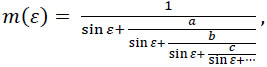
The mapping function, m (ε), is defined as the ratio of the electrical path length through the atmosphere at geometric elevation ε, to the electrical path length in the zenith direction. A mapping function is used to map the zenith delay to estimate the slant tropospheric delay. Several mapping functions have been developed in the past 20 years. The simplest mapping function is given by 1/sin(ε) [15], the cosecant of the elevation angle. In this derivation, it is assumed that spherical constant height surfaces could be approximated as planar surfaces. This is an accurate approximation only for high elevation angles and with a small degree of bending. More complex mapping functions have been developed, and different mapping functions may be used for the hydrostatic versus wet delays. Brief descriptions of the main features of various wet mapping functions are given in the following sub-sections.
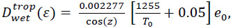
2.1. Saastamoinen Model
Saastamoinen developed a total delay model for the troposphere from which a “neutral” mapping function can be derived. It is given here because it can be applied for the wet delay as well as for the dry delay and has been popular among broad parts of the GPS user community in the past. Several stages of refinement exist for Saastamoinen's approach [16].
 |
(4) |
where,
z: apparent (“actual”) zenith angle at the surface (antenna),
ε: elevation angle (degree),
T0 : surface temperature in (K˚),
e0 : partial water vapor pressure in (mb).
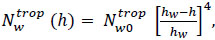
2.2. Hopfield Model
Hopfield used real data covering the whole Earth. He has empirically found a representation of the wet refractivity as a function of the height h above the surface by,
 |
(5) |
where, the mean value hw = 11000 m is used.
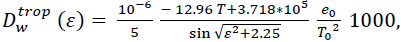
The result equations for wet components in (m) are [3];
 |
(6) |
where, T0 and e0 are measuring at the observation location and ε is the elevation angle.
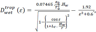
2.3. Black Model
The wet mapping functions derived by Black are based on the quartic profiles developed by Hopfield and use the equivalent heights proposed by Hopfield [3]. This mapping function was recommended for elevation angles above 5˚ and the slant wet delay is [17]:
 |
(7) |
where:
e0 : partial water vapor pressure at site in [mb],
T0 : temperature at site in [K˚],
Hw: upper boundary height for the wet delay/height of the tropopause,
r: radial distance from earth center to site,
ε: elevation angle in [degrees],
The Hw in eq. (7) can be approximated with help of surface temperature t0 as:
 |
(8) |
and the scale factor Lc in eq, (7) is:
| Lc = 0.167 - (0.076 + 0.00015 t0 ) .exp( -0.3 e). | (9) |
2.4. Chao Wet Mapping Function
Marini gave the elevation angle dependence of the atmospheric delay in the form a continued fraction, in terms of the sine of elevation angle ε [18]:
 |
(10) |
where, the coefficients a, b, c… are constants or linear functions which depend on surface pressure, temperature, lapse rates, and height.
In the Chao mapping functions, the continued fraction in eq. (10) is truncated to second order terms and the second order sin ε is replaced by tan ε, and the coefficients a and b are determined from empirical data. The wet mapping functions are expressed as follows [19]:
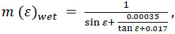 |
(11) |
2.5. Ifadis Wet Mapping Function
The global wet mapping function of Ifadis adopts the mapping function type [12]:
 |
(12) |
The wet mapping function coefficients are
a = 0.0005236 + 0.2471.10-6 (P0 - 1000) - 0.1724.10-6 (t0 - 15) + 0.1328.10-4 . 
b = 0.001705 + 0.7384.10-6 (P0 - 1000) - 0.3767.10-6 (t0 - 15) + 0.2147.10-4 .
c = 0.05917,
since,
P0 : pressure at site in [mb]
e0 : partial water vapor pressure at site in [mb]
t0 : temperature at site in [°C]
2.6. Herring Wet Mapping Function
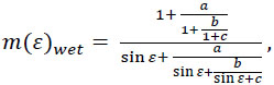
Herring has developed both hydrostatic and wet mapping functions by fitting to radiosonde data from several North American stations ranging in geographic latitude from 27˚ N to 65˚ N for elevation angles down to 3˚. The mapping function’s coefficients depend linearly on surface temperature, the cosine of the station latitude, and the height of the station above the geoid. The expression for the mapping function is given below [9]:
 |
(13) |
where, a, b, and c are constants or linear functions, and can be determined by:
a = [0.583 - 0.011 cosø - 0.000052 H0 + 0.0014 (t0 - 10)].10-3
b = [1.402 - 0.102 cosø - 0.000101 H0 + 0.0020 (t0 - 10)].10-3
c = [45.85 - 1.91 cosø - 0.00129 H0 + 0.015 (t0 - 10)].10-3
where:
t0 : temperature at site in [°C]
φ: latitude of site
H0 : height of site above sea level in [km]
2.7. Niell Wet Mapping Function
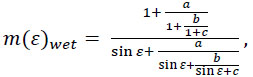
The Neill mapping functions have no parameterization in terms of meteorological conditions, and they provide a better fit and give better accuracy for elevation angles down to 3˚. The form adopted for the mapping functions is the continued fraction with three coefficients (a, b, c). The wet mapping function depends only on the site latitude [13]. The expressions for the wet mapping functions are given below:
 |
(14) |
where: ε is the elevation angle, and for the wet mapping function, only an interpolation in latitude for each parameter is needed. The average values of awet, bwet and cwet and their amplitudes are given in (Table 1).
| Coefficients | ɸ = 15˚ | ɸ = 30˚ | ɸ = 45˚ | ɸ = 60˚ | ɸ = 75˚ |
|---|---|---|---|---|---|
| a | 5.8021897e-4 | 5.6794847e-4 | 5.8118019e-4 | 5.9727542e-4 | 6.1641693e-4 |
| b | 1.4275268e-3 | 1.5138625e-3 | 1.4572752e-3 | 1.5007428e-3 | 1.7599082e-3 |
| c | 4.3472961e-2 | 4.6729510e-2 | 4.3908931e-2 | 4.4626982e-2 | 5.4736038e-2 |
2.8. Moffett Wet Mapping Function
Simplified approximations of the Hopfield mapping functions are presented in [20]. These simplified mapping functions have been used extensively, as they depend on the elevation angle only as in eq. (15):
 |
(15) |
2.9. Black and Eisner MF
The Black and Eisner mapping function for the total delay is a further modification of Black's, and is expressed as a simple geometrical model (16), which depends on the elevation angle only, with one fitted parameter [14]:
 |
(16) |
This mapping function is claimed to be valid for elevation angles greater than 7˚.
2.10. UNBabc MF
Jiming Gue and Richard B. Langley were produced a mapping Function called (UNBabc) had a 3-term continued fraction form as in eq. (10) [8]. From a series of analyses, they concluded that parameter (a) is sensitive to the orthometric height (H) and latitude (φ) of the station where as parameters b and c could be represented by constants. The least-squares estimated parameters for the wet mapping function:
aw = 0.61120 - 0.035348 H - 0.01526 cos φ / 1000
bw = 0.0018576
cw = 0.062741
The mapping functions assessed in this study and the corresponding codes and references used in the tables of results are listed in (Table 2).
| Code | Reference | Impute parameters | εmin˚ |
|---|---|---|---|
| SA | Saastamoinen (1987) | z, T0, eo | 10˚ |
| HO | Hopfield (1971) | ε, T0, eo | ** |
| BL | Black (1978) | ε, T0, eo, r | 5˚ |
| CH | Chao (1972) | ε | 10˚ |
| IF | Ifadis (1986) | ε, t0, eo, P0 | 2˚ |
| HE | Herring (1992) | ε, t0, φ, Ho | 3˚ |
| NI | Niell (1993) | ε, φ | 3˚ |
| MO | Moffett (1973) | ε | 2˚ |
| B & E | Black and Eisner (1984) | ε | 7˚ |
| UNBabc | Gue J. and Langley R. (2003), | ε, φ, H0 | 2˚ |
Saastamoinen model, Hopfield model and black model give the wet slant tropospheric delay directly but in other mapping functions used for the wet zenith tropospheric delay, the Saastamoinen model eq. (4) [21].
3. EXPERIMENTAL PROCEDURES
3.1. Research Methodology
Fig. (1) represents the flow chart followed in this Research. It contains several stages as follows:
 |
Fig. (1). Diagram of research methodology. |
1. Atmospheric modeling, it presents height profiles for pressure, temperature, and humidity.
2. Delay modeling, it aims to determine wet tropospheric delay at different zenith angles for three stations Aswan, Helwan, and Mersa-Matrouh in different times of year in Egypt (Numerical Integration Model).
3. Assessment of prediction models or mapping functions, this stage aims to determine best models and mapping functions which present high accuracy in wet tropospheric delay prediction for Egypt.
3.2. Ray Trace Model
In order to evaluate mapping functions, we ray-traced the refractivity profiles computed from the pressure, temperature and relative humidity profiles from balloon flights launched from 5 radiosonde stations at the Egyptian stations in the south of Egypt, near the Mediterranean Sea, and near the Red Sea over a period of 5 years (2000-2005). Most of the stations launched radiosonde twice daily, every day of the year.
When ray-trace methods are used to calculate range and elevation-angle errors, integrals for the bending, electromagnetic ray path, and the straight line path or geometric path (or the sums to which these integrals are reduced by layering) must be calculated for each of the many data points of a satellite pass. The integrals, moreover, must be calculated with great precision since the range error is calculated by taking the difference between the electromagnetic path and the geometric path, two nearly equal numbers.
In the method given by Thayer [22], the number of calculations required over a satellite pass is considerably reduced since the coefficients used to evaluate the integrals are independent of the elevation angle of the ray. The elevation angle at each layer must be calculated for each new ray by using Snell's law, however, and the need for great precision remains.
There are total of 1092 radiosonde profiles for the selected data set. For each profile, the ray tracing was done at elevation angles of 5˚, 6˚, 7˚, 8˚, 9˚, 10˚, 11˚, 13˚, 15˚, 17˚, 20˚, 25˚, 30˚, 35˚, 40˚, 45˚, 50˚, 55˚, 60˚, 65˚, 70˚, 75˚, 80˚, 85˚ and 90° to generate wet slant delays. The geographical distribution of the 5 stations is shown in [21]. The orthometric heights of the stations range from 32 m to 192 m slant wet tropospheric propagation delay are showed in (Figs. 2-4).
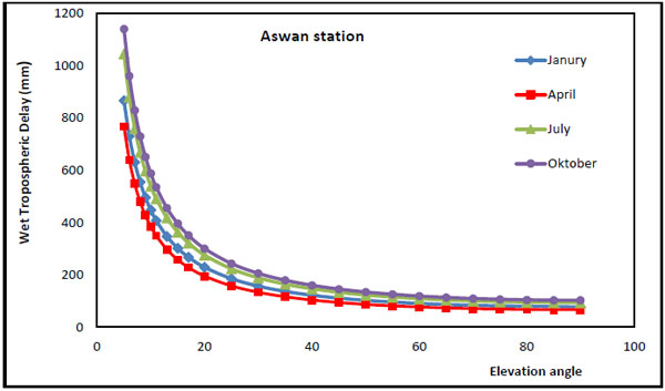 |
Fig. (2). Wet tropospheric propagation delay errors versus elevation angles at Aswan station (south of Egypt). |
 |
Fig. (3). Wet tropospheric propagation delay errors versus elevation angles at Helwan station (mid of Egypt). |
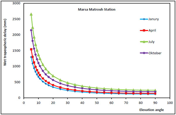 |
Fig. (4). Wet tropospheric propagation delay errors versus elevation angles at Marsa Matrouh station (north of Egypt). |
Analysis data received from ray-traced model showed that, wet tropospheric delay in Egypt varies from 66.84 mm to 223.34 mm at zenith and slant wet delay increase slowly with high elevation angles from 30˚ – 90˚. At elevation angle 60˚, wet delay error varies from min value 77.18 mm at Aswan station in April to max value 276.34 mm at Marsa Matrouh station in July month. For elevation angle 30˚, it changes from min value 133.69 at Aswan station in April to max value 478.29 mm at Marsa Matrouh station in July.
For the elevation angles lower than 30˚ the slant wet delay errors are increased suddenly. For elevation angles 15, wet delay error is 258.31 mm at Aswan station in April (min value) and 921.26 mm in July at Helwan station (max value). Wet delay errors at elevation angle 10 change from 385.09 mm to 1366.49 mm. for elevation angle 7; it arrives 1688.86 mm as min value but arrives 2323.43 mm as max value at elevation angle 5. Analysis of data in Figs. (2-4) resulted that wet tropospheric delay in Egypt increases from south of Egypt to Cairo region and increases near the Mediterranean Sea. Wet delay in Egypt in summer months is more than other seasons in middle and north of Egypt but in Upper Egypt max wet delay values are measured in autumn months.
3.3. Wet Delay MF
Slant delays are computed using the ray-traced vertical delays together with the ten mapping functions and compared to the ray-traced slant delays for elevation angles 5˚, 6˚, 7˚, 8˚, 9˚, 10˚, 11˚, 13˚, 15˚, 17˚, 20˚, 25˚, 30˚, 35˚, 40˚, 45˚, 50˚, 55˚, 60˚, 65˚, 70˚, 75˚, 80˚, 85˚, 90˚ at Aswan station, Helwan station and Marsa Matrouh station in January, April, July, October months and average data over the year.
4. RESULTS AND DISCUSSION
The results of the assessment are summarized in Tables (3-7) and the mean biases and rms errors of these mapping functions are showed in (Figs. 5-9).
| MF | Elevation angle 85˚ | Elevation angle 75˚ | ||||||
|---|---|---|---|---|---|---|---|---|
| min | max | mean | rms | min | max | mean | rms | |
| SA | 4.83 | 16.70 | 11.26 | 3.20 | 4.98 | 17.25 | 11.60 | 3.89 |
| HO | 9.04 | 30.19 | 18.02 | 5.24 | 9.33 | 31.15 | 18.59 | 5.40 |
| BL | 1.18 | -60.95 | -19.18 | 7.15 | 1.22 | -62.85 | -19.78 | 7.38 |
| CH | 4.86 | 16.72 | 11.25 | 3.29 | 5.02 | 17.25 | 4.60 | 3.39 |
| IF | 4.86 | 16.71 | 11.25 | 3.28 | 5.02 | 17.24 | 11.60 | 3.39 |
| HE | 4.86 | 16.72 | 11.25 | 3.28 | 5.02 | 17.24 | 11.60 | 3.39 |
| NI | 4.94 | 16.91 | 11.44 | 3.34 | 5.08 | 17.45 | 11.80 | 3.45 |
| M0 | 4.86 | 16.72 | 11.25 | 3.28 | 5.02 | 17.75 | 11.63 | 3.38 |
| B&E | 4.86 | 16.72 | 11.28 | 3.29 | 5.02 | 17.24 | 11.60 | 3.38 |
| UNBabc | 4.86 | 16.71 | 11.25 | 3.28 | 5.02 | 17.24 | 11.60 | 3.39 |
| MF | Elevation angle 60˚ | Elevation angle 45˚ | ||||||
|---|---|---|---|---|---|---|---|---|
| min | max | mean | rms | min | max | mean | rms | |
| SA | 5.55 | 19.23 | 12.93 | 3.78 | 6.80 | 23.49 | 15.78 | 4.61 |
| HO | 10.41 | 34.74 | 20.73 | 6.03 | 12.77 | 42.28 | 25.38 | 7.38 |
| BL | 1.35 | -70.10 | -22.07 | 8.23 | 1.60 | -86.08 | -27.03 | 10.08 |
| CH | 5.60 | 19.26 | 12.95 | 3.78 | 6.89 | 23.59 | 15.85 | 4.63 |
| IF | 5.60 | 19.25 | 12.95 | 3.78 | 6.90 | 23.61 | 15.87 | 4.63 |
| HE | 5.60 | 19.25 | 12.95 | 3.78 | 6.90 | 23.62 | 15.87 | 4.63 |
| NI | 5.68 | 19.48 | 13.17 | 3.85 | 7.00 | 23.89 | 16.14 | 4.72 |
| M0 | 5.60 | 19.25 | 12.95 | 3.78 | 6.89 | 23.58 | 15.85 | 4.63 |
| B&E | 5.60 | 19.27 | 12.96 | 3.79 | 6.94 | 23.72 | 15.95 | 4.66 |
| UNBabc | 5.60 | 19.25 | 12.95 | 3.78 | 6.90 | 23.62 | 15.87 | 4.64 |
| MF | Elevation angle 30˚ | Elevation angle 15˚ | ||||||
|---|---|---|---|---|---|---|---|---|
| min | max | mean | rms | min | max | mean | Rms | |
| SA | 9.62 | 33.00 | 22.19 | 6.48 | 21.44 | 69.53 | 46.42 | 13.55 |
| HO | 18.14 | 60.19 | 35.93 | 10.46 | 35.93 | 116.39 | 69.48 | 20.21 |
| BL | 2.31 | -121.18 | -38.15 | 14.21 | 4.33 | -232.23 | -73.108 | 27.72 |
| CH | 9.83 | 33.39 | 22.47 | 6.56 | 19.89 | 64.60 | 43.49 | 12.69 |
| IF | 9.90 | 33.58 | 22.59 | 6.60 | 20.56 | 66.75 | 44.95 | 13.12 |
| HE | 9.90 | 33.59 | 22.60 | 6.60 | 20.58 | 66.87 | 44.95 | 13.12 |
| NI | 10.04 | 33.97 | 22.98 | 6.71 | 20.87 | 67.40 | 45.66 | 13.32 |
| M0 | 9.83 | 33.37 | 22.45 | 6.56 | 19.92 | 64.69 | 43.56 | 12.71 |
| B&E | 10.06 | 34.02 | 22.91 | 6.69 | 22.02 | 70.69 | 47.74 | 13.92 |
| UNBabc | 9.91 | 33.60 | 22.61 | 6.60 | 20.67 | 66.88 | 45.07 | 13.15 |
| MF | Elevation angle 10˚ | Elevation angle 9˚ | ||||||
|---|---|---|---|---|---|---|---|---|
| min | max | mean | rms | min | max | mean | rms | |
| SA | 26.62 | 85.96 | 57.64 | 16.83 | 28.18 | 92.83 | 62.20 | 18.16 |
| HO | 55.67 | 173.77 | 103.79 | 30.19 | 62.77 | 193.03 | 115.32 | 33.54 |
| BL | 6.02 | -341.55 | -107.48 | 40.07 | 6.53 | -377.01 | -118.61 | 44.23 |
| CH | 31.73 | 96.38 | 64.93 | 18.93 | 36.16 | 106.80 | 72.09 | 21.01 |
| IF | 34.07 | 103.80 | 69.94 | 20.39 | 39.36 | 117.10 | 78.93 | 23.00 |
| HE | 34.16 | 104.27 | 70.00 | 20.42 | 39.49 | 117.76 | 79.03 | 23.05 |
| NI | 34.51 | 104.03 | 70.95 | 20.69 | 39.98 | 117.88 | 80.03 | 23.33 |
| M0 | 31.95 | 85.7 | 65.38 | 19.06 | 35.65 | 107.99 | 72.80 | 21.22 |
| B&E | 38.99 | 117.11 | 79.38 | 23.12 | 46.06 | 135.25 | 91.80 | 26.73 |
| UNBabc | 34.41 | 104.22 | 70.33 | 20.50 | 39.81 | 117.66 | 79.46 | 23.15 |
| MF | Elevation angle 7˚ | Elevation angle 5˚ | ||||||
|---|---|---|---|---|---|---|---|---|
| min | max | mean | rms | min | max | mean | rms | |
| SA | 30.39 | 108.05 | 72.18 | 21.08 | 24.05 | 115.64 | 76.52 | 22.47 |
| HO | 84.86 | 248.50 | 148.60 | 43.21 | 118.36 | 350.53 | 210.13 | 61.06 |
| BL | 7.78 | -474.64 | -149.15 | 55.68 | 9.63 | -633.12 | -197.99 | 74.21 |
| CH | 50.45 | 137.16 | 92.51 | 26.94 | 83.21 | 190.63 | 128.85 | 37.44 |
| IF | 57.03 | 157.96 | 106.57 | 31.04 | 99.61 | 242.27 | 163.81 | 47.67 |
| HE | 57.37 | 159.49 | 106.92 | 31.16 | 100.69 | 246.85 | 165.22 | 48.13 |
| NI | 55.65 | 158.67 | 107.94 | 31.43 | 87.64 | 246.97 | 165.69 | 48.18 |
| M0 | 46.26 | 140 | 94.49 | 27.50 | 66.64 | 200.90 | 136.01 | 39.51 |
| B&E | 70.89 | 195.52 | 133.20 | 38.76 | 134.74 | 359.11 | 231.47 | 67.35 |
| UNBabc | 57.94 | 159.08 | 107.63 | 31.33 | 101.82 | 245.10 | 166.42 | 48.38 |
 |
Fig. (5). Mean difference of the wet tropospheric delay errors between the delays computed using the mapping functions and the ray trace results for elevation angles from 30˚ to 90˚. |
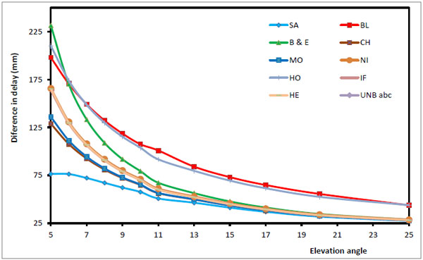 |
Fig. (6). Mean difference of the wet tropospheric delay errors between the delays computed using the mapping functions and the ray trace results for elevation angles from 5˚ to 30˚. |
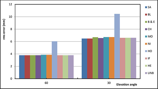 |
Fig. (7). Root mean square wet tropospheric delay errors about the mean of the differences between the delays computed using the mapping functions and the ray trace results for 30˚ and 60˚ elevation angles. |
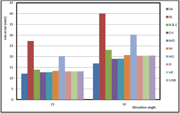 |
Fig. (8). Root mean square wet tropospheric delay errors about the mean of the differences between the delays computed using the mapping functions and the ray trace results for 10˚ and 15˚ elevation angles. |
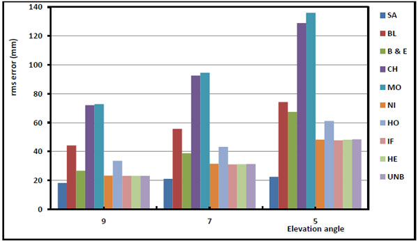 |
Fig. (9). Root mean square wet tropospheric delay errors about the mean of the differences between the delays computed using the mapping functions and the ray trace results for 5˚, 7˚ and 9˚ elevation angles. |
For elevation angles above 30˚, virtually all mapping functions except Hopfield MF and Black wet delay model yield errors of less than 23 mm with rms errors no more than 7 mm. for elevation angle 30˚, mean error difference between Hopfield MF and ray-trace model arrives 35.93 mm with rms 10.46 mm but for Black wet delay model the mean difference is -38.15 mm and rms is 14.21 mm, means that the Hopfield model and Black wet delay model is not citable for atmospheric conditions of Egypt. From analysis of the figures, SA, CH, IF, HE, NI, MO, B & E and UNBabc mapping functions provide sub-centimeter accuracy for angles above 15˚ with minimum difference between them no more than 4 mm in mean difference and 2 mm in rms values. For elevation angles below 10˚, only a few of the functions are found to adequately meet the requirements currently imposed by space geodetic techniques.
The SA, CH and MO mapping functions are quite accurate at elevation angles above 10˚. Since, at elevation angle 10˚, the mean difference for SA mapping functions arrives 57.64 mm with rms 16.83 mm, and 64.93 mm with rms 18.93 mm for CH mapping functions and 65.38 mm with rms 19.06 mm for MO mapping functions. For low elevation angles less than 10˚, The Saastamoinen mapping functions perform well. However, the mean difference by SA mapping function compared to the ray tracing for the data set used at elevation angle 7˚ is 76.52 mm with rms 22.97 mm and 76.52 mm with rms 22.97 mm for elevation angle 5˚, comparing with 92.51 mm with rms 26.94 mm for CH mapping functions at 7˚ elevation angle and 128.85 mm with rms 37.44 mm at elevation angle 5˚.
Both the Hopfield and Black mapping functions differences with respect to ray tracing indicate some seasonal and/or latitudinal dependence. This might be caused by the use of nominal values for the tropopause height and temperature lapse rate. However, it seems likely that such nominal values will be used in space geodetic software since values of such parameters for specific sites and atmospheric conditions are generally not exactly known.
Table 8 summarizes the best five mapping functions based on the mean difference, rms and relative error as compared to the delay computed using ray trace model for Egypt. For this data set, the Saastamoinen, Chao, Moffett, Ifadis and Herring mapping functions provided the same level of accuracy for elevation angle more than 10˚. For elevation angle less than 10˚, as can be seen in Table 8b, and 8c, the Saastamoinen, Chao and Moffett functions consecutively place first, second and third, respectively. The results states that if information is available on the vertical temperature and water vapor pressure distribution in the atmosphere, the Saastamoinen mapping function should be used. Otherwise, one of the mapping functions derived by Chao and Moffet should be used.
| a) 30˚ elevation angle | 15˚ elevation angle | ||||||||
|---|---|---|---|---|---|---|---|---|---|
| MF | Mean difference | rms | Percent error | rank | MF | Mean difference | rms | Percent error | rank |
| SA | 22.19 | 6.48 | 8.24 | 1 | CH | 43.49 | 12.69 | 8.39 | 1 |
| MO | 22.45 | 6.56 | 8.34 | 2 | MO | 43.56 | 12.71 | 8.40 | 2 |
| CH | 22.47 | 6.56 | 8.35 | 3 | IF | 44.95 | 13.12 | 8.67 | 3 |
| IF | 22.59 | 6.60 | 8.39 | 4 | HE | 44.95 | 13.12 | 8.67 | 4 |
| HE | 22.60 | 6.60 | 8.40 | 5 | UNB | 45.07 | 13.15 | 8.70 | 5 |
| b) 10˚ elevation angle | 9˚ elevation angle | ||||||||
| MF | Mean difference | rms | Percent error | rank | MF | Mean difference | rms | Percent error | rank |
| SA | 57.64 | 16.83 | 7.50 | 1 | SA | 62.20 | 18.16 | 7.31 | 1 |
| CH | 64.93 | 18.93 | 8.45 | 2 | CH | 72.09 | 21.01 | 8.46 | 2 |
| MO | 65.38 | 19.06 | 8.51 | 3 | MO | 72.80 | 21.22 | 8.55 | 3 |
| IF | 69.94 | 20.39 | 9.10 | 4 | IF | 78.93 | 23.00 | 9.27 | 4 |
| HE | 70.00 | 20.42 | 9.11 | 5 | HE | 79.03 | 23.05 | 9.28 | 5 |
| c) 7˚ elevation angle | 5˚ elevation angle | ||||||||
| MF | Mean difference | rms | Percent error | rank | MF | Mean difference | rms | Percent error | rank |
| SA | 72.18 | 21.08 | 6.65 | 1 | SA | 76.52 | 22.47 | 5.13 | 1 |
| CH | 92.51 | 26.94 | 8.52 | 2 | CH | 128.85 | 37.44 | 8.63 | 2 |
| MO | 94.49 | 27.50 | 8.71 | 3 | MO | 136.01 | 39.51 | 9.11 | 3 |
| IF | 106.57 | 31.04 | 9.82 | 4 | HE | 165.22 | 48.13 | 10.97 | 4 |
| HE | 106.92 | 31.06 | 9.85 | 5 | IF | 163.81 | 47.67 | 11.07 | 5 |
The SA, CH, and Moffett mapping functions are quite accurate at very low elevation angles (less than 10˚) than the other mapping functions as compared to the ray tracing for the data set used. Therefore, for high-precision applications, it is recommended that the mapping function derived by Saastamoinen model be used as the first choice. The second choice will be the Chao or the Moffett mapping function.
CONCLUSION
From the presented results, we have concluded that the wet component of the slant tropospheric delay can be predicted with sub-millimeter accuracy, using the Saastamoinen model, provided accurate measurements of surface meteorological data or site dependent parameters are available.
In spite of the large number of mapping functions we have analyzed, only a small group meet the high standards of modern space geodetic data analysis: Chao, Moffett, Ifidas and Herring mapping functions.
For elevation angle above 15, SA, CH, MO, IF, HE, NI, UNB and B&E yield identical mean biases and the best total error performance. At lower elevation angles, SA, CH, MO, IF and HE are clearly superior. As regards the rms scatter about the mean, Saastamoinen mapping function performs the best for all elevation angle, followed closely by Chao and Moffett mapping functions respectively.
CONFLICT OF INTEREST
The authors confirm that this article content has no conflict of interest.
ACKNOWLEDGEMENTS
This work was not completed without the help of many other people. Firstly, my professors at public works department, they have provided me with more opportunities than I could have imagined. Thank you for believing in me, supporting me, and helping me along the way.
Also, the financial contribution of all members of the Egyptian Meteorological Authority for preparing, realizing and analyzing the measurements of temperature, pressure and humidity with different heights within their authority.
Finally, and most importantly, Sarah, for their love and support for all of my friends, students and laboratory for putting up with me while I prepared this paper.